Network morphology
Beyond its topology, a pore network also carries the morphology of the void space: the size of every pore and every throat. PoreScene can map such a per-element property onto the stick-and-ball geometry, coloring each sphere and cylinder by its own value and compositing a matching colorbar, so the pore- and throat-size distribution can be read straight off the render.
This example loads a pore network from a MATLAB file, configures its radius property
with a colormap, and builds the stick-and-ball geometry. It then renders the network
twice: once with every pore and throat colored by radius, and once with the pores hidden
and the solid phase added, so the throats can be seen running through the material they
connect.
This tutorial builds on the network topology example and reuses the same pore network extracted from the freeze-dried sugar solution captured with X-ray micro-computed tomographic imaging [1], available in PoreScene’s repository on GitHub: data/pnm.mat
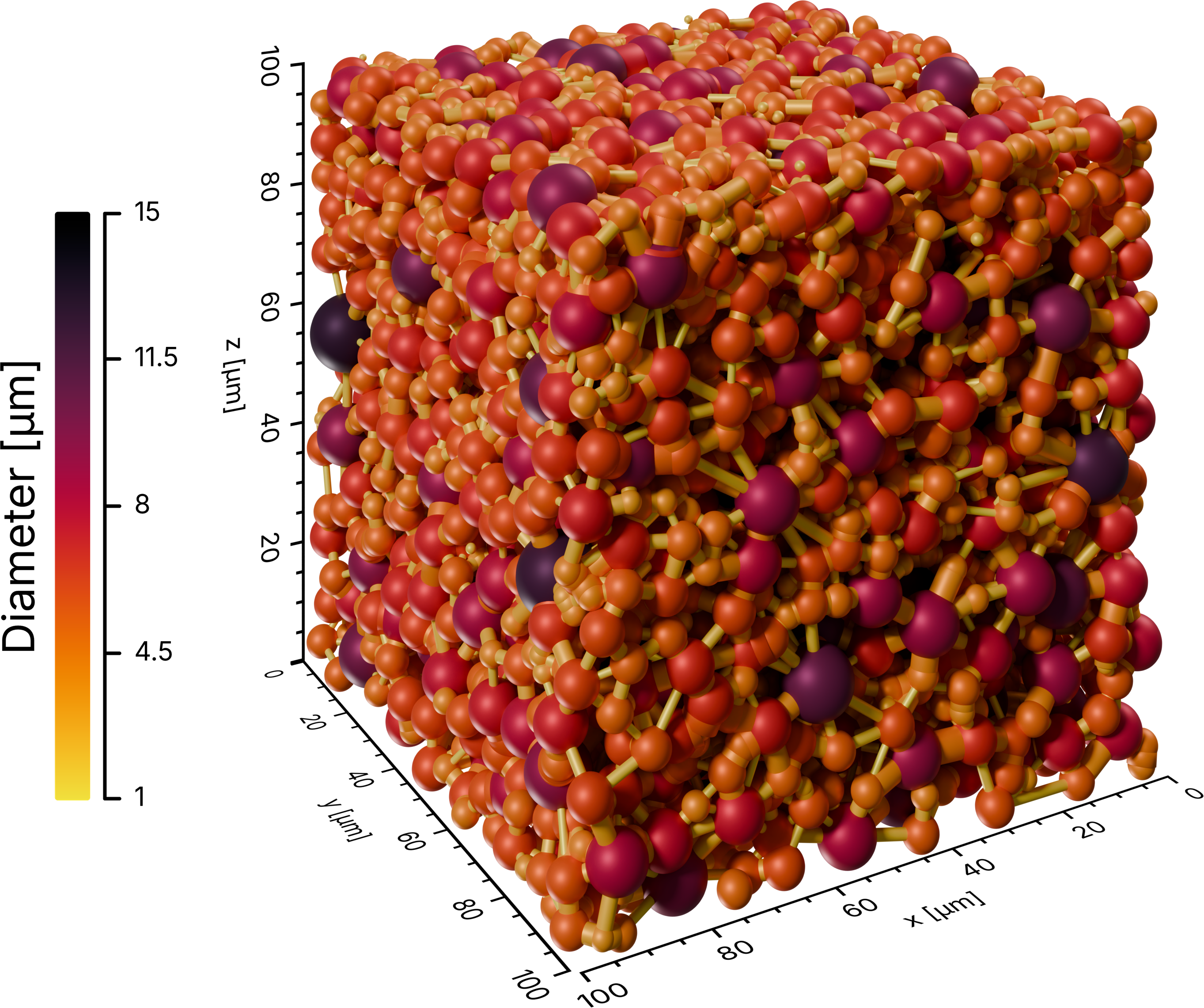
The first render: the pore network in stick-and-ball representation, with every pore and throat colored by its radius, on-scale axes and the matching colorbar.
Step-by-step guide
1. Import required modules
Make sure to have porescene installed (see Installation). At first, required modules need to be imported:
import json
from pathlib import Path

from porescene import worker
from porescene.color.palette import Colormap, Palette
from porescene.config import PropertyConfiguration
from porescene.model import PoreNetwork
from porescene.scene import Scene
from porescene.utility import CompassDirection, Orientation
PoreNetwork holds the pore and throat data, while
Scene sets up the rendering stage. Module
worker provides the high-level helpers that build the stick-and-ball
geometry and render it colored by radius. Palette and
Colormap supply the gradient colors, and
PropertyConfiguration describes how the radius property is
colored and labelled – with Orientation and
CompassDirection placing the colorbar. File paths and
directories are handled throughout PoreScene with the built-in pathlib module, and
json reads the variable mapping.
2. Set utility variables
After that, the directory holding the input data and receiving the rendered images is specified:
# data directory
pth_data = Path.cwd() / "data"
pth_data holds the input files – the pore network and the solid mesh – and also
receives the rendered images together with their colorbars.
3. Load the pore network
The network is stored in a MATLAB file. Because the variable names inside such a file
differ from project to project, from_mat() takes a
mapping from PoreScene’s attribute names to the variable names in the file. That mapping
lives in map_vars.json and is loaded first:
# load variable mapping for variable import from .mat file
with open(pth_data / "map_vars.json") as f:
    map_vars = json.load(f)

# load pore network data from MAT file
pn = PoreNetwork.from_mat(pth_data / "pnm.mat", map_vars["data_network"])
The loaded PoreNetwork carries the pore positions and radii,
the throat radii, and the throat-to-pore connectivity that PoreScene needs to place the
spheres and cylinders. Unlike the network topology example, the
imported radii are kept as they are – they are exactly the property this example colors
by.
4. Scene setup
The scene is created directly from the physical extent of the network, which sizes it
and calibrates the axes to the real dimensions of the sample (see Concepts & Conventions):
# initialize a new scene
sc = Scene(pn.extent)
Tip
To reuse a saved camera, lighting and axis configuration instead of the defaults, load
it from a PoreScene JSON file with
Scene.from_json().
Next, the radius property is registered on the scene. A
PropertyConfiguration names the property – the name
make_radius() looks it up by later – and gives its gradient the
colors to interpolate, here the EMBER colormap in reverse via
Palette.load(...).reversed():
# initialize PNM property "radius"
sc.config_scene.add_property(
    PropertyConfiguration(
        "radius",
        Palette.load(Colormap.EMBER).reversed(),
        heading="Diameter [µm]",
        orientation=Orientation.VERTICAL,
        align=CompassDirection.WEST,
        precision=0,
        factor=2e6,  # converts radius in [m] to diameter in [µm]
    )
)
The remaining arguments shape the colorbar: heading sets its title, orientation
and align stand it vertically on the west (left) side, and precision fixes the
number of decimals on its tick labels. factor scales only the values printed on the
colorbar, not the geometry: 2e6 turns a radius in meters into a diameter in
micrometers (2 for radius to diameter, 1e6 for meters to micrometers), which is
why the heading reads Diameter [µm].
Tip
Any member of Colormap can be dropped in here. For a
continuous property such as the radius, a perceptually uniform sequential colormap
keeps equal steps in value looking like equal steps in color, and its hue progression
stays readable across the shaded spheres and cylinders. Reversing it with
reversed() simply flips which end of the range
is which color.
build_structure() then builds the stick-and-ball geometry, one
sphere per pore and one cylinder per throat. Calibrated axes are added around it:
# add cylinders and spheres to the scene
worker.build_structure(sc, pn)

# add axes around the scene
sc.create_axes()
5. Render by radius
make_radius() does the coloring in one call: it fits a smooth
gradient to the combined pore- and throat-radius range, colors the sphere and cylinder
layers accordingly, renders the scene, trims the image, and composites the colorbar
described by the radius property. The result is written into pth_data:
# render the scene and color pores and throats according to their radius
pth_img = worker.make_radius(pth_data, pn, sc)
This first render is the stick-and-ball view shown at the top of the page: every pore and
throat carries its own color from the reversed EMBER gradient, next to the matching
colorbar and the on-scale axes.
6. Solid and throats only
The same scene is now reused for a second view that swaps the pore spheres for the solid
phase, so the throats can be seen running through ^the pore space of the material. The meshed
solid from the solid structure example is added, the sphere layer is
switched off in the scene configuration, and the radius gradient is re-pointed at a
different colormap by reassigning its
colors:
# add a solid object to the scene
sc.create_solid(pth_data / "solid.ply")

# disable the pore spheres so only the solid and throats remain
sc.config_scene.enable_spheres = False

# change the colormap for radius property
sc.config_scene["radius"].colors = Palette.load(Colormap.SPEED).all()
Because make_radius() shows and colors a layer only when it is
enabled in the scene configuration, disabling the spheres leaves just the throats – now
colored by the SPEED gradient – threaded through the solid. A second call renders
that view:
# render the scene and color the throats according to their radius
pth_img = worker.make_radius(pth_data, pn, sc)
Note
Every render resets the scene afterwards – hiding the pore, throat and cluster layers and removing the solid. The two renders are named after the layers they show (spheres and cylinders for the first, solid and cylinders for the second), so neither overwrites the other.
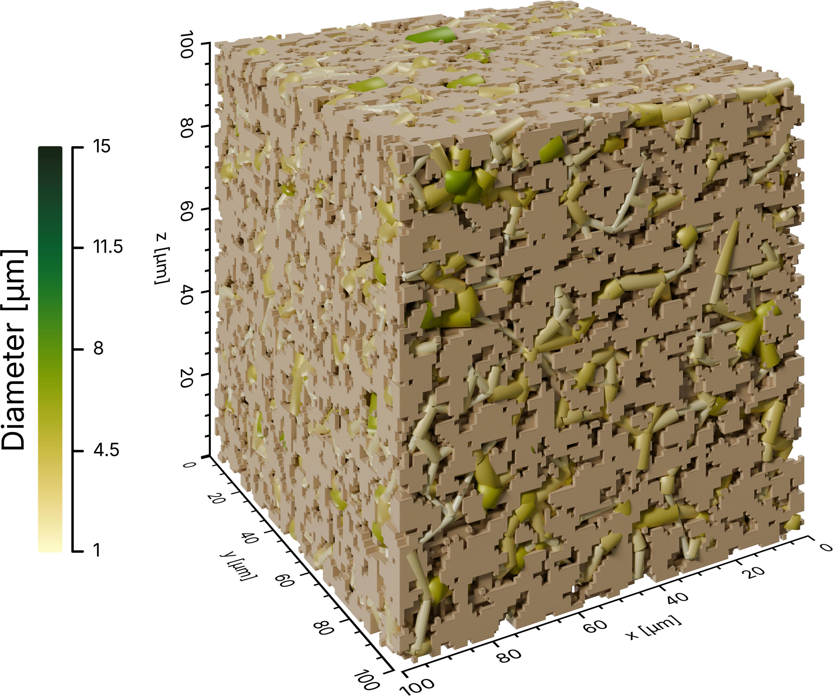
The second render: the pore spheres hidden and the solid phase added, leaving the cylinders – still colored by their radius – running through the material they connect.
Full script
The complete example, also available on GitHub: example/network_morphology.py.
 1import json
 2from pathlib import Path
 3
 4from porescene import worker
 5from porescene.color.palette import Colormap, Palette
 6from porescene.config import PropertyConfiguration
 7from porescene.model import PoreNetwork
 8from porescene.scene import Scene
 9from porescene.utility import CompassDirection, Orientation
10
11# =============================================================================
12# Import Parameters
13
14# data directory
15pth_data = Path.cwd() / "data"
16
17
18# =============================================================================
19# Scene configuration
20
21# load variable mapping for variable import from .mat file
22with open(pth_data / "map_vars.json") as f:
23    map_vars = json.load(f)
24
25# load pore network data from MAT file
26pn = PoreNetwork.from_mat(pth_data / "pnm.mat", map_vars["data_network"])
27
28# initialize a new scene
29sc = Scene(pn.extent)
30
31# initialize PNM property "radius"
32sc.config_scene.add_property(
33    PropertyConfiguration(
34        "radius",
35        Palette.load(Colormap.EMBER).reversed(),
36        heading="Diameter [µm]",
37        orientation=Orientation.VERTICAL,
38        align=CompassDirection.WEST,
39        precision=0,
40        factor=2e6,  # converts radius in [m] to diameter in [µm]
41    )
42)
43
44# add cylinders and spheres to the scene
45worker.build_structure(sc, pn)
46
47# add axes around the scene
48sc.create_axes()
49
50
51# =============================================================================
52# Render pores and throats colored by radius
53
54# render the scene and color pores and throats according to their radius
55pth_img = worker.make_radius(pth_data, pn, sc)
56
57
58# =============================================================================
59# Render the solid with throats only
60
61# add a solid object to the scene
62sc.create_solid(pth_data / "solid.ply")
63
64# disable the pore spheres so only the solid and throats remain
65sc.config_scene.enable_spheres = False
66
67# change the colormap for radius property
68sc.config_scene["radius"].colors = Palette.load(Colormap.SPEED).all()
69
70# render the scene and color the throats according to their radius
71pth_img = worker.make_radius(pth_data, pn, sc)